Introduction
This is an abridged summary of the bowtie image classification process that only highlights the key points.
Silicon photovoltaic wafers are cut from silicon inguts using a wire saw. The wire sawing process introduces saw damage in the form of residual stress and microcracks near the wafer surfaces. Locally elevated shear stresses are observed in regions near microcracks. The locally elevated shear stress fields resemble the shape of a bowtie when observed with the aid of an infrared grey-field polariscope (IR-GFP); hence the name "bowtie defect".
This post focuses on the process of identifying bowtie defects in microscopic IR-GFP images. Eight ML classifiers were optimized and trained to classify bowtie defects in infrared images.
Using the XGBClassifier (extreme gradient boosting classifier) a recall value of 96% with a precision of 87% was achieved resulting in an F1 score of 0.913. This performed better than the soft classifier when uniformly weighted and when weighted according to each classifiers peak F1 score. Only by heavily weighting the soft voter were similar results to the XGB classifier produced.
Bowtie defects in microscopic IR-GFP images. Image width ≊ 400 μm.
Summary of Steps
All subheadings can be clicked to reveal more details.
[1-4] Post processing raw IR-GFP image data:
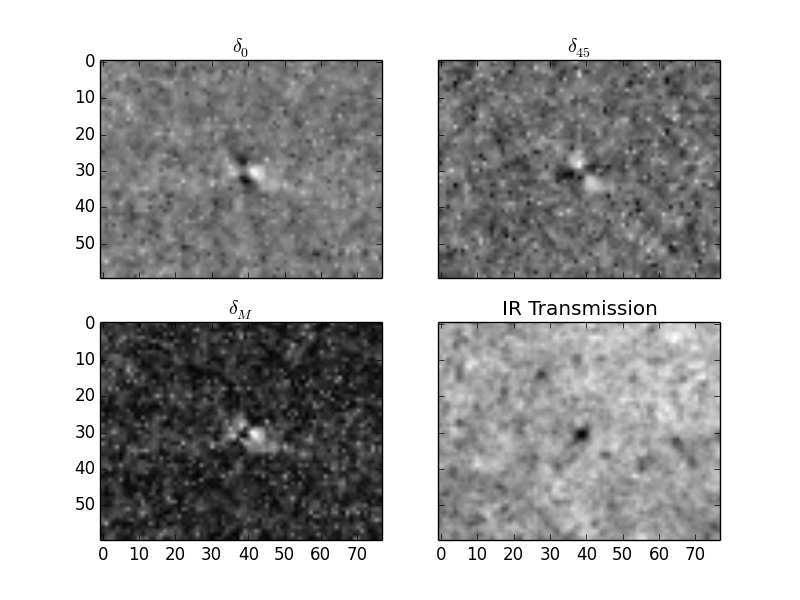
- converting .dt1 (Delta Vision) files into Shear 0, Shear 45, and Shear Max images
- creating/applying subtraction images
- detecting (and removing) hypersensitive pixels and unnecessary images
- identifying (and ignoring) low quality images
[5-8] Creating two machine learning (ML) training sets for identifying bowties:
- img: standard deviation and numpy arrays of shear 0 and shear 45 images
- circlescan: standard deviation and circle sweep of shear 0 and shear 45 images
- circle sweep: (a.k.a. circle scan) a list of points where each point is the average value of a 20 micron radial line scan from the center of a bowtie, where the line scan is swept tangentially about the center of the bowtie
[9] Optimize 8 ML classifiers:
- Extra Trees Classifier (using img and circlescan training sets)
- Random Forest Classifier (using img and circlescan training sets)
- Support Vector Classifier (using img and circle scan training sets)
- Extreme Gradient Boosted Classifier (using img training set)
- Extreme Gradient Boosted Random Forest Classifier (using img training set)
[10] Combine classifier output though weighted soft voting:
- Uniformly weighted and weighted according to each classifiers peak F1 score
[11] Demonstrate the best model's ability to classify bowties:
- XGB Classifier outperforms soft voter
Details
Most subheadings can be clicked to reveal more details.
[1] Collect light level information from each microscopic image and track which pixels have outlier intensity values.
This information will be used to filter out low quality images and identify hypersensitive pixels. Hypersensitive pixels are pixels that consistently have higher than true values as a result of thermal effects, they occur more frequently after prolonged imaging sessions.
[2] Calculate the distribution of light intensity from the 3,500 images that make up each wafer.
These values will be used to filter out low quality microscopic IR-GFP images based on average light level and standard deviation of pixel intensities.
[3] Identify hypersensitive pixels.
The probability of any single pixel having the greatest value in a 640 by 480 array more than 4 times out of 3,500 images is very small. Identify the pixels that fit this description and remove them. Recursively repeat this process until no hot pixels remain.
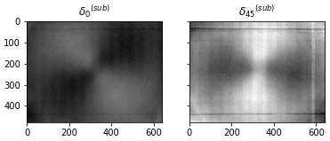
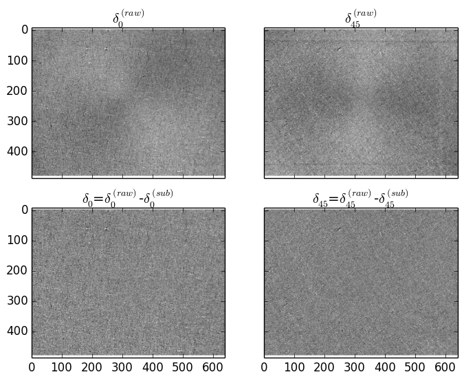
[4] Generates a shear 0 and shear 45 subtraction image for each wafer.
A subtraction image is the average of 108 images and will be used to remove the effects of consistent optical aberrations caused by reflections, imperfections in the optic train, and a polychromatic light source. Low quality images (images of the wafer mask or blurry images) are filtered out prior to selecting the 108 images that will be used to make the subtraction image. Of the remaining images, the 108 images with the lowest average shear max retardation are selected to make the subtraction image.
Example Subtraction Image
Effect of Applying Subtraction Image
[5] Annotate 5x IR-GFP images to facilitate the process of identifying bowties. Manually identified bowties and nonbowties will be used to train the machine learning classifier.
Shear 0 Manual Bowtie Identification

Shear 45 Manual Bowtie Identification

[6] Preprocess 40 by 40 pixel regions of interest that have been manually identified as bowtie or non-bowtie. This eases the process of extracting features from the sample data in the next step.
[7-8] Extract 2 training data sets from the preprocessed images. The purpose of using multiple training datasets is to create more diverse classifiers so that they can benefit from each other through soft voting.
- Circle Sweep
- A radial line scan is swept in a circle around the image to create an array of the average line scan value at various angles.
- This focuses on features related to the profile of the bowtie.
- Flattened Array
- Flattens the 8 by 8 pixel region about the center of the bowtie to a 1D array.
[9] Train and optimize eight classifiers (4 for each set of training data):
- Data Split: training (80%), testing (20%)
- XGB Data Split: training (64%), validation (16%), testing (20%)
- SVMs: transformers use a standard scaler to prevent outliers from skewing the data
- Random Forest: no scaler used - it is not necessary
- Parameters considered during the optimization process:
- XGBC: gamma, learning_rate, max_depth, reg_lambda, early stopping
- XGBRFC: learning_rate, max_depth, min_child_weight, subsample, colsample_bynode, reg_lambda
- SVC: kernel, gamma, C, number of features, size of max pool
- RFC: max_depth, bootstrap, min_samples_leaf, max_features
- ETC: max_depth, bootstrap, min_samples_leaf, max_features
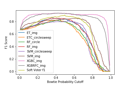
[10] Compare the classifiers: (click to show details)
Each classifier is capable of predicting the probability of each instance being a bowtie or nonbowtie. A soft voting classifier takes into account the predicted probabilities from all of the classifiers when calculating the probability that an instance is a bowtie. Each classifier can be either equal weight ('uniform') or be weighted according to how well the classifier performed on its own ('f1' or 'f1pow'). Where 'f1pow' skews the soft voter's decisions towards the best individual classifier.- The performance of the classifiers was calculated individually and using the soft voting method
- With regard to the soft voter's performance: 'f1pow'>'f1'>'uniform'
- As evident below, the XGBClassifier performed the best
- As the power of 'f1pow' is increased the soft voter's F1 curve will gradually approach XGB_img classifier's F1 curve
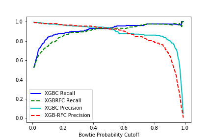
The XGBClassifier and XGBRFClassifier outperformed all of the other classifiers considered here. Below are the precision vs threshold and recall vs threshold plots for the xgboost classifiers, where threshold is the critical predicted probability a classifier must have to classify an instance as a bowtie.
For this project having a high recall value is more important than having a high precision value. This is because the goal is to characterize wafer strength according to the distribution of microcracks on each wafer. Missing a critical microcrack would be more detrimental to the goal than accidentally characterizing a nonbowtie as a bowtie. Thus the recommended bowtie probability threshold is 0.8 because for higher threshold values there is very little gain in recall and a severe decrease in precision.
Using a threshold value of 0.8 with the XGBClassifier a recall value of 96% with a precision of 87% is achieved resulting in an F1 score of 0.913.
[11] Apply the classifier to new 5x IR-GFP images. Image is divided into equal sized subimages. The most intense pixel in each subimage is classified as either a bowtie (positive) or nonbowtie (negative). Positive classifications are boxed in white and negative classifications are boxed in black. Bowties are annotated according to the subimage number.
Adjust the subimage size to match the density of defects.